My friend Eliška got a cake from Merci chocolate bars and Ferrero Rocher, attached to a base from polystyrene. It was really finely done, with satisfactory geometric regularity.

That got us thinking: how does one even estimate, which base size to buy, not knowing how many Merci pieces fit around its circumference.
The first step is to measure a width of Merci piece, $m$, which is fixed (at least until the next shrinkflation). Based on my measurements in Linz, Austria on 23 March 2025, $m=1.9$ cm.
m = 1.9 # merci width
Next, we tile a circle of radius $r$ with $k$ Merci pieces -- both $r$ and $k$ are unknown. We want to keep the tiling of the circumference as perfect as possible, i.e., minimize the remaining gap $\epsilon\in[0,m)$ where the bar cannot fit anymore as small as possible.
Models
Circular model
The first model simplifies Merci to an arc of the length $m$ on the circle of the sought radius $r$.
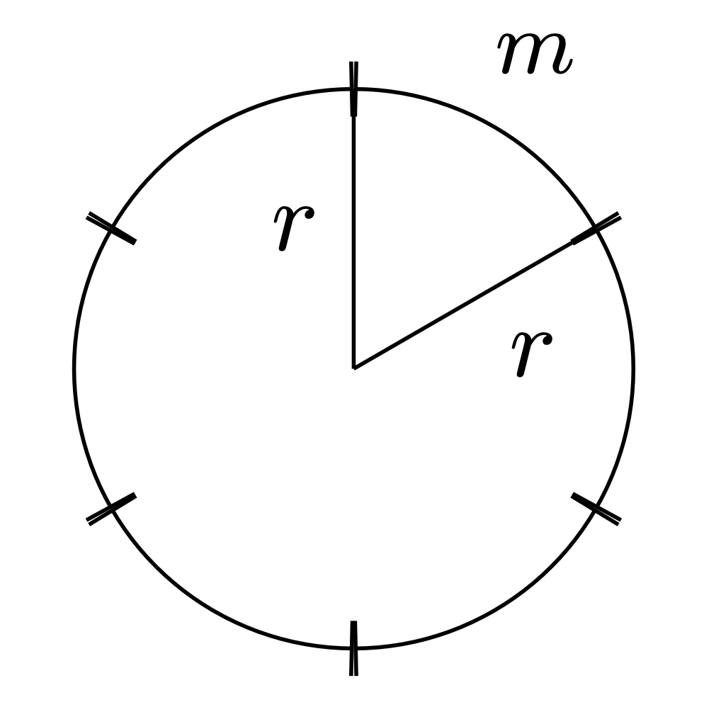
This implies $k$ Mercis reach the length of $k m$ and the total length is $2\pi r$. The full model along with the tiling gap is
$$ 2\pi r=k\cdot m+\epsilon. $$
We can actually directly estimate $k$ as $k=\lfloor\frac{2\pi r}{m}\rfloor$. For the $k$ estimate, we then calculate the gap $\epsilon$.
Polygon model
Our second attempt is a polygon model with the circular base inscribed inside.
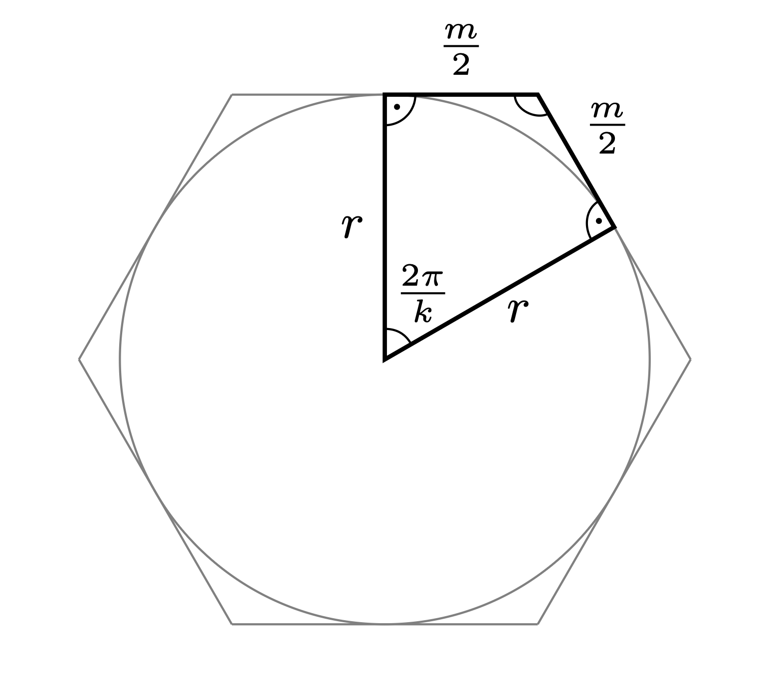
This way, we express the relationship of $m$ and $k$ as
$$ \tan\left(\frac{\pi}{k}\right)=\frac{m}{2r}. $$
We convert this to arc lengths, to allow for the tiling gap $\epsilon$ as before.
$$ 2\pi r = 2kr\arctan\left(\frac{m}{2r}\right)+\epsilon. $$
Results
We assess the quantization error over different choices of $r$ and $k$.
import numpy as np
import pandas as pd

df = []
for r in np.arange(4.5,6.5,.1):
    k1 = int(np.floor(2*np.pi*r / m))
    k2 = int(np.floor(np.pi / np.atan(m/2/r)))
    df.append({
        'r': r,
        'circ0': 2*np.pi*r,
        'm': m,
        # circle model

        'k1': k1,
        'eps1': 2*np.pi*r - k1*m,
        'circ1': k1*m,
        # polygon model

        'k2': k2,
        'eps2': 2*np.pi*r - 2*k2*r * np.atan(m/2/r),
        'circ2': 2*k2*r * np.atan(m/2/r),
    })
df = pd.DataFrame(df)
The results for both models are presented in the table below.
| $r$ | $2\pi r$ | $k_\circ$ | $k_\circ m$ | $\epsilon_\circ$ | $k_{\text{⬡}}$ | $2k_{\text{⬡}}r\arctan(\frac{m}{2r})$ | $\epsilon_{\text{⬡}}$ |
|---|---|---|---|---|---|---|---|
| 4.5 | 28.274 | 14 | 26.6 | 1.674 | 15 | 28.088 | 0.187 |
| 4.6 | 28.903 | 15 | 28.5 | 0.403 | 15 | 28.105 | 0.798 |
| 4.7 | 29.531 | 15 | 28.5 | 1.031 | 15 | 28.121 | 1.410 |
| 4.8 | 30.159 | 15 | 28.5 | 1.659 | 16 | 30.012 | 0.147 |
| 4.9 | 30.788 | 16 | 30.4 | 0.388 | 16 | 30.027 | 0.760 |
| 5.0 | 31.416 | 16 | 30.4 | 1.016 | 16 | 30.042 | 1.374 |
| 5.1 | 32.044 | 16 | 30.4 | 1.644 | 17 | 31.934 | 0.110 |
| 5.2 | 32.673 | 17 | 32.3 | 0.373 | 17 | 31.948 | 0.725 |
| 5.3 | 33.301 | 17 | 32.3 | 1.001 | 17 | 31.961 | 1.340 |
| 5.4 | 33.929 | 17 | 32.3 | 1.629 | 18 | 33.854 | 0.076 |
| 5.5 | 34.558 | 18 | 34.2 | 0.358 | 18 | 33.866 | 0.692 |
| 5.6 | 35.186 | 18 | 34.2 | 0.986 | 18 | 33.877 | 1.308 |
| 5.7 | 35.814 | 18 | 34.2 | 1.614 | 19 | 35.771 | 0.043 |
| 5.8 | 36.442 | 19 | 36.1 | 0.342 | 19 | 35.782 | 0.660 |
| 5.9 | 37.071 | 19 | 36.1 | 0.971 | 19 | 35.793 | 1.278 |
| 6.0 | 37.699 | 19 | 36.1 | 1.599 | 20 | 37.687 | 0.012 |
| 6.1 | 38.327 | 20 | 38.0 | 0.327 | 20 | 37.697 | 0.630 |
| 6.2 | 38.956 | 20 | 38.0 | 0.956 | 20 | 37.707 | 1.249 |
| 6.3 | 39.584 | 20 | 38.0 | 1.584 | 20 | 37.716 | 1.868 |
| 6.4 | 40.212 | 21 | 39.9 | 0.312 | 21 | 39.611 | 0.602 |
Practical assessment
TBD